Abstract

With an emphasis on regular and unique kernels, this abstract delves into the numerical solution of second class Volterra integral equations. The second kind of Volterra integral equations are a common type of equations in many practical domains, such as engineering and physics. The intricacy of solving these equations stems from the fact that the kernel might be either smooth (regular) or have singularities; the integral involving the unknown function defines them. When analytical solutions are not possible, computational methods become very important in solving these equations, as the abstract emphasizes. For efficient approximation of solutions, methods including numerical integration, iterative schemes, and discretization techniques (e.g., collocation and Galerkin methods) are used. Conventional numerical approaches provide quite accurate results when applied to regular kernels, but singular kernels necessitate additional handling, typically through transformation or adaptive grids, in order to deal with their single behaviour. The computational method addresses the problems presented by solitary kernels and the ways to overcome them, with an emphasis on the importance of accuracy and efficiency, especially for problems of a large scale.

Keywords: Solution, Approach, Equation, Integral, Numerical method.

Introduction

A set of integral equations known as Volterra integral equations of the second kind finds extensive use in many branches of science and technology, from engineering and biology to economics and physics. An integral over a known kernel function defines the unknown function f (t), which is at the heart of these equations. To be more precise, the second kind of Volterra integral equation is,

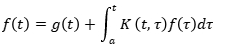
The known function g (t) and the variable K (t, τ), which might change depending on the specific problem, are the equation’s kernels. The fact that the unknown function shows up both within and outside the integral gives rise to the name “second kind” equation. It is common practice to use complex computational methods to find solutions to these equations over a certain interval [a, b], particularly in cases when the kernel K (t, τ) has particular characteristics like regularity or singularity.

Research into numerical solutions to Volterra integral equations, and more specifically, the second sort, is essential, especially when considering issues with practical applications. Because these equations are not always easy to solve analytically, computational approaches are now essential. By approximating the solution in a reasonable form, numerical approaches provide valuable insight into complicated systems. Dealing with the nature of the kernel function is an important part of numerically solving these equations.

Volterra integral equations typically use either a regular or singular kernel. Smooth and well-behaved kernels over the integration domain are called regular kernels. Typical techniques, such as the trapezoidal rule or Simpson’s rule, are usually enough for computing the integral in these instances. In contrast, singular kernels add complexity because of how they act at certain points, usually when t is close to τ. These kernels might act in ways that make numerical integration difficult, such as being unbounded or having undefined values at specific locations. To deal with these singularities properly, specialist methods are needed.

Discrete optimization is a common computing strategy for solving regular kernel Volterra integral equations. The quadrature rules, which evaluate the integral at a small number of places to approximate it, are one of the most frequent ways to break the continuous integral into a finite sum. Solving the resulting system of linear equations using well-established techniques such as iterative solvers, LU decomposition, or Gaussian elimination is possible after discretization. But extra caution is required when the kernel is solitary. Modifications to numerical methods are often necessary when dealing with singular kernels. These modifications can include the use of singular quadrature methods or the use of regularization techniques to reduce the impact of the singularity. A regularization term can be included to smooth out the singular kernel and enable stable numerical integration, which is one way to deal with these singularities.

For the second sort of Volterra integral equations, discretization is not the only approach; the sequential approximation method and the Neumann series expansion are also frequently used. When solving linear Volterra equations, the iterative approximation of the unknown function by repeated corrections is facilitated by the Neumann series approach. The idea behind this approach is to iteratively improve the approximation by expanding the solution as an integral series. Similarly, one well-known iterative strategy is the successive approximation method, which involves iteratively refining an initial answer guess by solving a series of simpler problems.

When dealing with single kernels, techniques like spline-based approaches or generalized quadrature can be used to manage integration during intervals where the kernel becomes unbounded. In order to increase the numerical solution’s correctness, these methods frequently utilize adaptive techniques and localize the kernel’s behavior. In order to make numerical integration concentrate on regions where the kernel shows singularities, adaptive methods change the step sizes according to the solution and kernel behavior.

Computational approaches for regular and singular kernel Volterra integral equations have recently seen substantial improvements in accuracy and performance. The capacity to tackle these problems on large scales has been further improved by advances in adaptive algorithms, parallel computing, and error analysis, allowing the application of these techniques to increasingly complicated, real-world settings.

To sum up, a crucial yet difficult topic of computational mathematics is the numerical solution of second-kind Volterra integral equations, especially those involving regular and unique kernels. To get good approximations to these equations, one can use a variety of techniques, such as discretization, iterative methods, and singular kernel specialized approaches. Our capacity to answer more and more complicated Volterra integral equations will increase in tandem with the development of more powerful computers and more efficient algorithms, opening us new avenues of inquiry and potential solutions in many fields.

Review of Related Studies

Adeyemi, Olagunju & Ibrahim, Adebisi. (2024). Numerical solutions of the Volterra integral equations are discussed in this article. A novel strategy for using the spectral method is suggested, with a basis function that is a first-kind Chebyshev polynomial (x T k). Coefficients of (x T k) in the residual equations are equated to generate system of equations in the approach of series solution, which is the fundamental basis of the method. An expression for the estimated mistakes is found, which can be used as a cap on the total amount of errors. We provide numerical examples on a few standard integral equations to show how well the method works and how accurate its error estimates are.

Bhat, Imtiyaz & Mishra, Lakshmi. (2022). This paper proposes an approach to numerically solving the third class of Volterra integral equations (VIEs) using approximations based on the Lagrange polynomial, modified Lagrange polynomial, and barycentric Lagrange polynomial. This is accomplished by thinking about the unknown function’s interpolation in terms of the polynomials mentioned earlier, which have unknown coefficients. An equation system involving linear algebra is produced by inserting this approximation into the equation under consideration. We next show that the approach converges and that it can estimate errors. All of these methods keep the solution’s potential singularity in mind. Researchers have not yet tackled the singularity case, as far as the authors are aware. At the end, we offer examples with both symmetric and non-symmetric kernels to show how new methods work and how accurate they are for the suggested integral equation.

Zarnan, Jumah. (2018). Using a numerical approach provided, this study numerically solves second-kind Volterra integral equations with regular and unique kernels. We compare the numerical solution to the existing method in the literature and look at numerical examples to make sure the proposed derivations work.

Fariborzi Araghi, Mohammad et al., (2008). Our approach involves utilizing the discrete Gronwall inequality, the Euler Maclaurin summation formula, variable transforms, a modified version of Simpson’s integration rule, and Navot’s quadrature to resolve the second-class singular Abel integral problem. Nonlinear weakly singular Volterra integral equations can be solved using the proposed approach. Next, we deduce the algorithm’s convergence. The effectiveness and precision of the aforementioned approach are demonstrated by a few numerical outcomes.

Maleknejad, Khosrow et al., (2008). The numerical solution of second-kind (VK2), first-kind (VK1), and even singular-type Volterra integral equations is introduced in this study. Using Bernstein’s approximation to approximate an unknown function is the foundation of the suggested approach. This approach uses straightforward computation to get an approximation that is satisfactory. In addition, we obtain a bound estimate for the method’s error. We give various instances to demonstrate the efficacy of this strategy.

Maleknejad, Khosrow et al., (2003). The method developed by M. Razzaghi and S. Yousefi is applied to solve linear second kind integral equations using continuous Legendre wavelets on the interval [0,1]. For the purpose of approximating the integral equations, we compute the inner products of all functions using the quadrature formula. We proceeded to simplify the integral equation by reducing it to solutions of algebraic linear equations.

Preliminaries

An integral equation in 𝑎(𝑥) often takes the form

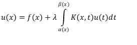
The integral equation (1) has a kernel 𝐾 (𝑥, 𝑏) and the limits of integration are 𝛽(𝑥) and 𝛽(𝑥). The integral sign makes the unknown function 𝑏(𝑥) readily apparent. Please take note that in equation (1), 𝜇 is a constant parameter and both the kernel 𝐾 (𝑥, 𝑡) and the function 𝑓(𝑥) are provided functions.

The form is the most common representation of the Volterra integral equations.

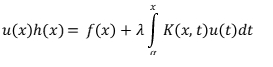
where the integral sign is used to describe a linear relationship between 𝑥 and the unknown function 𝑏(𝑥), and the limits of integration are functions of 𝑥. When the function ℎ(𝑥) equals 1, equation (2) is reduced to a simple form.

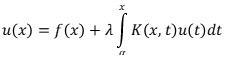
The second class of Volterra integral equations are these; however, equation (2) changes to

Which belongs to the first class of integral equations and is called the Volterra category.

Results of Solution Method

The problem is referred to as being of the convolution type and may be solved using the Laplace transform, which provides the exact solution of Volterra integral equations, when the kernel of the equation is of the difference form [𝐾 (𝑥 − 𝑦)]. In order to resolve the second sort of Volterra integral equations, the researchers employed a straightforward and effective Galerkin weighted residual numerical approach that utilized Chebbyshev polynomials as the trial function.

The numerical approach for solving the second sort of Volterra integral equations using the trapezoidal rule is presented in this study.

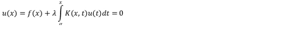
Here we present a numerical technique for solving the second kind of Volterra integral equations. Consider again the equation.

The following equation results from first approximating the integral term in the equation using the trapezoidal rule:

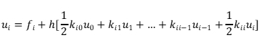
The approximate answer to can be found from this equation:(3) at𝑢(𝑥𝑖)=𝑢1, where𝑥𝑖=𝑎+𝑖ℎ, 𝑖=1, 2, 𝑛; 𝑓𝑖=𝑓(𝑥𝑖)and𝐾𝑖j=𝐾 (𝑥𝑖, 𝑡j) =0𝑓𝑜𝑟𝑡j>𝑥𝑖.

It is possible to express the approximate solution (5) as 𝑍 equations in𝑢𝑖at𝑥𝑖=𝑎 +𝑖ℎ, 𝑖=1, 2, 𝑛, since𝑢𝑜=𝑓₀is considered the starting point. The equation system is

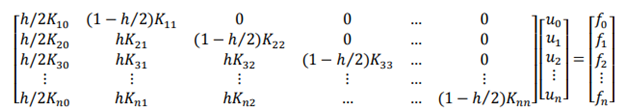
The answer can be found by repeatedly substituting 𝑏0 as the beginning point for forward substitution.

Conclusion

While numerically solving second-kind Volterra integral equations, especially with regular and unique kernels, is a major obstacle in computational mathematics, it provides crucial resources for solving many real-world problems in many different domains. Given the form of these integral equations, precise solutions can only be obtained by using specialist methods. This is particularly true when the kernel function displays particular behaviors, such regularity or singularity. We can now deal with these equations much more effectively in real-world situations, thanks to the invention and implementation of numerous computer approaches.

The numerical solution is made easier when the kernel is regular. To get a good approximation of the integral in the equation, one can use quadrature techniques or other traditional numerical integration methods. A direct solution can be found by discretizing the integral problem into a system of linear equations. Reliable methods for this process include iterative solvers or Gaussian elimination. Careful discretization and proper numerical integration techniques are typically necessary for these methods to work, as they guarantee that the approximation will converge to the genuine solution within acceptable error ranges. Accuracy and computing efficiency in large-scale tasks demand advanced strategies like adaptive step sizes or parallel processing; yet, normal kernels’ simplicity shouldn’t be overlooked.

Statements & Declarations:

Peer-Review Method: This article underwent double-blind peer review by two external reviewers.

Competing Interests: The author/s declare no competing interests.

Funding: This research received no external funding.

Data Availability: Data are available from the corresponding author on reasonable request.

Licence: Numerical Solution of Volterra Integral Equations of the Second Kind with Regular and Singular Kernels: A Computational Approach © 2026 by Kumar, Pawan & Pal, Rajiv is licensed under CC BY-NC-ND 4.0. Published by IJABS.

References:

1. Adeyemi, , & Ibrahim, A.(2024). Numerical solution of Volterra integral equation and its error estimates via spectral method.
2. Baratella, P., & Orsi, A. P.(2004). A new approach to the numerical solution of weakly singular Volterra integral equations. Journal of Computational and Applied Mathematics, 163(2), 401–418. https://doi.org/10.1016/j.cam.2003.08.047
3. Bhat, A., & Mishra, L. N.(2022). Numerical solutions of Volterra integral equations of third kind and its convergence analysis. Symmetry, 14(12), 2600. https://doi.org/10.3390/sym14122600
4. Brunner, H., Pedas, A., & Vainikko, G.(1999). The piecewise polynomial collocation method for nonlinear weakly singular Volterra equations. Mathematics of Computation, 68(227), 1079–1095. https://doi.org/10.1090/S0025-5718-99-01073-X
5. Diogo, , Lima, P., & Rebelo, M. (2005).Computational methods for a non linear Volterra integral equation, Proceeding of hermca.
6. Fariborzi Araghi, A., & Daei Kasmaei, H. (2008). Numerical solution of the second kind singular Volterra integral equations by modified Navot-Simpson’s quadrature. International Journal of Open Problems in Computer Science and Mathematics. IJOPCM, 3.
7. Liu, -P., & Tao, L. (2007).Mechanical quadrature methods and their extrapolations for solving first kind Abel integral equations. Journal of Computational and Applied Mathematics, 201(1), 300–313. https://doi.org/10.1016/j.cam.2006.02.021
8. Lubich, Ch.(1985). Fractional Linear multistep methods for Abel–Volterra integral equations of the second kind. Mathematics of Computation, 45(172), 463–469. https://doi.org/10.1090/S0025-5718-1985-0804935-7
9. Lyness, J. N., & Ninham, B. W.(1967). Numerical quadrature and asymptotic expansions. Mathematics of Computation, 21(98), 162–178. https://doi.org/10.1090/S0025-5718-1967-0225488-X
10. Maleknejad, , Hashemizadeh, E., & Ezzati, R.(2011). A new approach to the numerical solution of Volterra integral equations by using Bernstein approximation. Communications in Nonlinear Science and Numerical Simulation, 16(2), 647–655. https://doi.org/10.1016/j.cnsns.2010.05.006
11. Maleknejad, , Tavassoli Kajani, M., & Mahmoudi, Y.(2003). Numerical solution of linear Fredholm and Volterra integral equations of the second kind by using Legendre Wavelets. Kybernetes, 32(9/10), 1530–1539. https://doi.org/10.1108/03684920310493413
12. Monegato, G., & Schuderi, L.(1998). High order methods for weakly singular integral equations with non smooth functions. Mathematics of Computation, 1493–1515.
13. Navot, (1962).A further extension of Euler-Maclaurin summation formula. Journal of Mathematics and Physics, 41(1–4), 155–163. https://doi.org/10.1002/sapm1962411155
14. Tao, , & Yong, H. (2003).A generalization of discrete Gronwall inequality and its application to weakly singular Volterra integral equation of the second kind. Journal of Mathematical Analysis and Applications, 282(1), 56–62. https://doi.org/10.1016/S0022-247X(02)00369-4
15. Tao, , & Yong, H. (2006).Extrapolation method for solving weakly singular nonlinear Volterra integral equations of the second kind. Journal of Mathematical Analysis and Applications, 324(1), 225–237. https://doi.org/10.1016/j.jmaa.2005.12.013
16. Zarnan, (2018). Numerical solution of Volterra Integral equations of second kind.

Cite this Article:

Kumar, P., & Pal, R. (2026). Numerical solution of Volterra integral equations of the second kind with regular and singular kernels: A computational approach. International Journal of Applied and Behavioral Sciences, 3(1), 153–161. https://doi.org/10.70388/ijabs250169