Abstract
This paper presents the Higher-Order Haar Wavelet Collocation Method (HHWCM), an advanced numerical technique designed to address the limitations of the traditional Haar Wavelet Collocation Method (HWCM). By incorporating higher-order polynomial extensions into the Haar wavelet framework, the proposed method enhances precision and achieves faster convergence rates. The HHWCM is developed to effectively solve nonlinear ordinary differential equations (ODEs) under a wide array of conditions, including initial conditions, boundary conditions, periodic conditions, two-point conditions, integral conditions, and multi-point integral boundary conditions. The study begins with a theoretical foundation of HHWCM, demonstrating its improved approximation capabilities through convergence analysis and error estimation. This study underscores the versatility and potential of HHWCM as a robust computational tool for addressing nonlinear differential equations in scientific and engineering applications. The findings open avenues for extending the method to partial differential equations (PDEs) and exploring its integration with machine learning techniques to enhance numerical modelling and simulation in future work.
Keywords: Numerical method, Wavelet, Non-linear, Convergence, Collocation.
Introduction
Because of their remarkable skills in solving complicated mathematical problems, such as differential and integral equations, wavelet methods have become an important tool in numerical analysis. The simplest of these wavelet families, Haar wavelets are well-known for being computationally efficient and for being able to manage solutions with severe discontinuities. The collocation approach has become popular because it is easy to use, efficient, and can adapt to all kinds of boundary conditions when paired with Haar wavelets. To meet the need for improved accuracy and convergence in solving nonlinear differential equations, this work enhances the classical Haar wavelet collocation approach and applies it to its higher-order variations.
All sorts of disciplines rely on nonlinear differential equations to explain complicated systems, from physics and engineering to biology and beyond. Nevertheless, getting analytical solutions might be challenging due to their intrinsic nonlinearity, which calls for robust numerical approaches. By combining the precision and adaptability of higher-order formulations with the power of wavelet theory, the higher-order Haar wavelet collocation method offers a fresh perspective. This technique incorporates higher-order terms to enhance resolution and accuracy, capitalizing on the compact support and orthogonality of Haar wavelets.
To tackle nonlinearities and discontinuities in complicated systems, the suggested higher-order Haar wavelet collocation method improves convergence rates and boosts accuracy compared to conventional methods. The approach ensures more accurate approximation by capturing tiny details of the solution and increasing the resolution of the wavelet basis. The fact that it can deal with boundary-layer phenomena and non-uniform grids makes it a very useful tool for solving practical problems.
The convergence characteristics, computational efficiency, and accuracy in solving nonlinear differential equations are the main points of this study, which focuses on the creation and implementation of the higher-order Haar wavelet collocation method. Using examples involving boundary layers, equations with singularities, and other difficult aspects, the paper shows how the method can be applied. This study’s overarching goal is to prove that the higher-order Haar wavelet collocation method is a solid strategy for contemporary computer mathematics by tackling these critical points.
REVIEWS OF RELATED WORK
Hussain, Basharat & Afroz, Afroz. (2022) The authors introduce a novel numerical method for approximating the solutions of SPDDEs, or simultaneous proportional delay differential equations. This technique takes use of collocation points and delayed Haar wavelet series to convert SPDDEs into an algebraic matrix equation system where the coefficient matrices are unknown. Find the values of these unknown row matrices with the help of a good solver. In terms of collocated Haar wavelet series, the solution is derived using these coefficients. In addition, the method’s suitability, efficacy, and applicability are investigated by a numerical experiment on linear and non-linear systems.
Karkera, Harinakshi & Katagi, Nagaraj. (2021) This work examines the constant two-dimensional flow of a viscous fluid as a result of a stretching sheet in a magnetic field. We offer two novel numerical approaches for addressing the governing problem represented by the Falkner-Skan equation, which are based on the Haar wavelet in conjunction with a collocation approach and a quasi-linearization process. We compute the significant derived numbers that represent the fluid velocity and wall shear stress for different values of the flow parameters M and β. Previous results did not account for lesser values of the magnetic parameter (M < 1), negative β, and nonlinear stretching parameters; nevertheless, the suggested approaches allow us to achieve these answers. It is clear from the numerical and graphical results that the created methods are efficient and accurate, and they also display a strong agreement with the existing findings. One major benefit of this method over previous semi-analytical and numerical approaches is that it doesn’t rely on beginning assumptions and small parameters.
Qasim, Ahmed & S. Al-Rawi, Ekhlass. (2021) Analytical determination of the integrals of the suggested formula is carried out in this research, which derives a new wavelet formula from the definition of the convolution between the Haar and CAS wavelets. The collocation sites for solving partial differential equations are outlined in the suggested method. We found that the proposed method is superior, more accurate, and closer to an exact answer after comparing the numerical results of three problems with the precise solution.
Shiralashetti, Siddu & Hanaji, Savita. (2021) This study presents a numerical method based on Hermite wavelets that can solve the non-linear Benjamina-Bona-Mohany partial differential equation with two parameters that is singularly perturbed. The current approach relies solely on the collocation technique for time discretization of Hermite wavelet series approximations. Two famous equations, the singly perturbed non-linear Benjamina-Bona-Mohany partial differential equation with two parameters, and other situations are used to test the efficacy of the suggested technique. We offer numerical solutions based on Hermite wavelets at various time levels in figures and tables, and compare them to exact and known techniques of solution. The matlab codes for the proposed method are also provided. The correctness and usefulness of the suggested method are demonstrated by the presentation of figures and tables that contain the computed absolute error at different time levels.
Singh, Inderdeep. (2019) This paper presents a numerical approach to solving generalized Burger’s type equations that is both efficient and effective. The initial step in solving the generalized Burger’s type equations is to change the wave variables such that they become nonlinear ordinary differential equations. Applying the quasilinearization method, linearize these nonlinear differential equations. The collocation approach based on Haar waves is utilized for solving systems of linear equations that are algebraic. One unique thing about the suggested approach is how easily it can be used for different kinds of nonlinear partial differential equations in two and three dimensions. To demonstrate the precision and effectiveness of the suggested approach, numerical trials are carried out.
Arora et al., (2018) This work presents a novel hybrid method that uses wavelets to solve nonlinear and higher-order linear boundary value problems. A family of non-dyadic wavelets with a dilation factor of 3 is used to approximate the answer in the suggested method. Using the collocation method, the domain is discretized. The quasi-linearization method is used to solve boundary value problems with nonlinearities. On order ranging from eight to twelfth, eleven numerical experiments are conducted on linear and nonlinear boundary value problems to demonstrate the effective implementation of the suggested approach. In order to demonstrate the method’s superiority over alternative approaches, the resulting solutions are also compared with exact and numerical solutions published in the literature.
Arora (2018) An innovative hybrid approach based on wavelets is introduced in this paper for solving nonlinear and higher-order linear boundary value problems. The method proposed works by approximating the solution using a non-dyadic wavelet family with a dilation factor of 3. Subdomains are created by dividing a domain using the collocation method. When dealing with boundary value difficulties, quasi-linearization is employed to tackle nonlinearities. Eleven numerical experiments on nonlinear and linear boundary value problems with orders between eight and twelve demonstrate the efficiency of this strategy. The results are compared with the exact and numerical answers published in the literature to further demonstrate the method’s efficiency.
ShijuJin (2018) The main emphasis of this work is a collocation spectral method for 2D Sobolev equations. A 2D Chebyshev polynomial collocation spectral model is constructed for these equations before proceeding to more complicated issues. After that, we check if the spectral numerical solutions exist, are unique, stable, and converge. Theoretical changes are then backed by numerical experiments. Based on these findings, it seems that the collocation spectrum model is a great tool for numerically solving 2D Sobolev equations.
HAAR WAVELETS
When it comes to wavelets, the Haar wavelet is among the most basic kinds utilized in signal processing. Its defining feature is a basis that resembles a step function; this basis partitions the data into subregions, enabling time- and frequency-domain localization analysis. The computational efficiency and simplicity of the Haar wavelet transform make it ideal for data compression, edge detection, and image processing applications.
Definition of Haar Wavelet
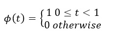
Two functions, ϕ(t) for scaling and ψ(t) for wavelet transformation, are utilized to define the Haar wavelet:
- Scaling Function (ϕ(t))
- Wavelet Function (ψ(t))
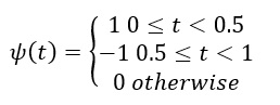
Through signal change detection, the wavelet function extracts the “high-frequency” information.
Haar Wavelet Transform
By using the Haar wavelet transform, a signal can be broken down into its detail and approximation coefficients. At each stage, the process is repeated repeatedly, dividing the signal in half:
- Approximation coefficients (A) stand for the mean of neighbouring signal levels.
- Detail coefficients (D) identify the discrepancy between neighbouring signal values.
Assume a separated signal to be . In its computations, the Haar wavelet transform
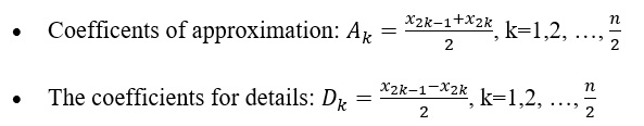
A multilevel decomposition can be formed by applying the transform again to the approximation coefficients.
Properties of Haar Wavelets
- Compact Support: The computational efficiency of the Haar wavelet is due to the fact that its non-zero values only fall inside a limited interval.
- Orthogonality: No redundancy in the decomposition is ensured by the orthogonality of the Haar wavelet and scaling functions.
- Simple Structure: For signals with abrupt changes, its step-like form is perfect, and it’s also easy to implement.
Applications of Haar Wavelets
- Image Compression: Utilized in methods such as JPEG 2000 for the purpose of image compression using coefficient representation.
- Edge Detection: Records abrupt changes in signal or picture quality to assist with edge identification.
Signal Denoising: Filters out background noise from signals without losing any of the useful information.
HAAR COLLOCATION WAVELET METHOD
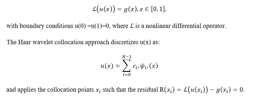
To solve differential equations, integral equations, and other mathematical problems, the numerical methodology known as the Haar collocation wavelet method combines Haar wavelets with collocation methods. It shines when precision is paramount or when dealing with issues with intricate boundary conditions. Technique for Collocation. As a numerical technique, the collocation method uses a collection of basic functions to approximate a function, which is the solution to a differential or integral problem. At some discrete locations known as collocation points, the differential equation is satisfied.
Using Haar wavelets as foundation functions, the collocation sites are usually selected as the midpoints of the subintervals created by the wavelets in the Haar collocation wavelet method.
Steps in the Haar Collocation Wavelet Method
- Problem Setup
- Think about the standard form of a differential or integral equation:
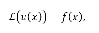
- inside the bounds of the known function f(x) and the operator L.

- Add the estimate to the governing equation:

- Determine the coefficients by solving the system of equations using normal numerical methods (such as LU decomposition or Gaussian elimination) .
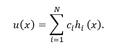
- Build the solution u(x) using the wavelets and coefficients:
Haar wavelet collocation methods
The two distinct HWCMs were shown here.
Haar wavelet collocation method based on Chen and Hsiao approach
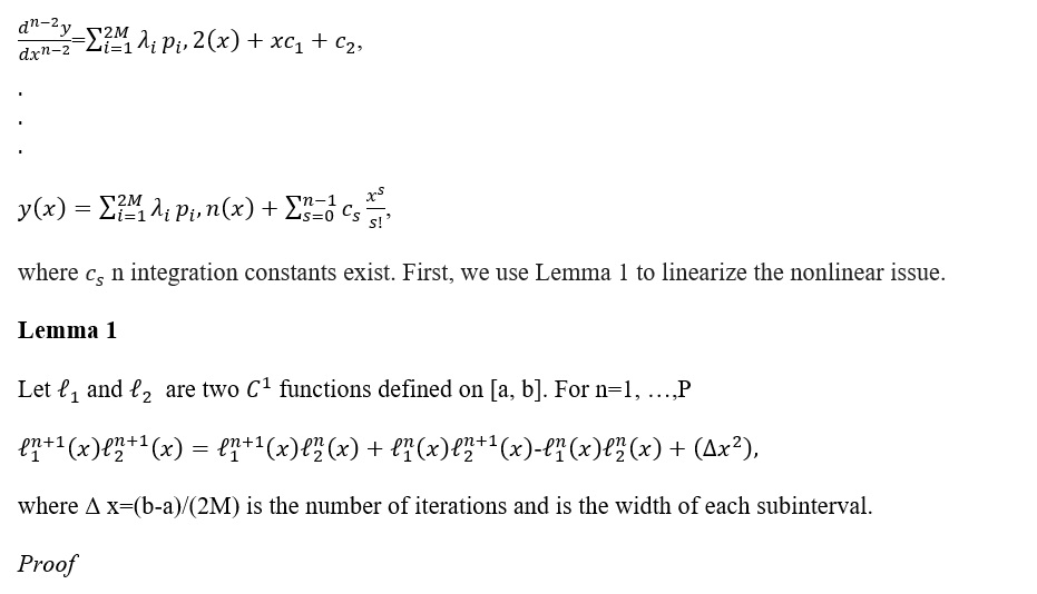
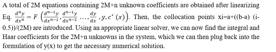
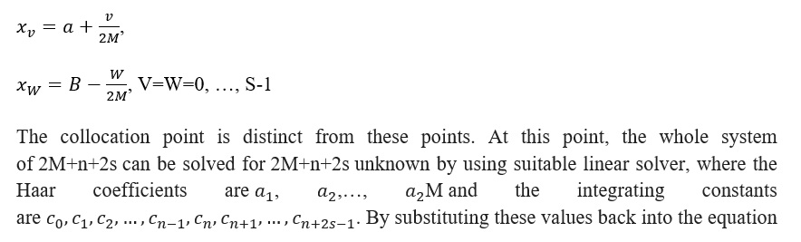
Several HWCMs have been developed in the past 20 years to solve integro-differential and differential problems. Although they employ different integration techniques and algorithms, all of these HWCMs adhere to the methodology put forth by Chen and Hsiao. Rather than trying to estimate the solution term, the highest-order derivative in the model is instead approximated using the Haar series, as per the technique outlined by Chen and Hsiao. We approximation in order to answer ![]() for instance.
for instance.


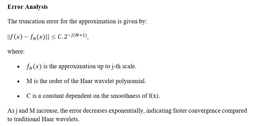
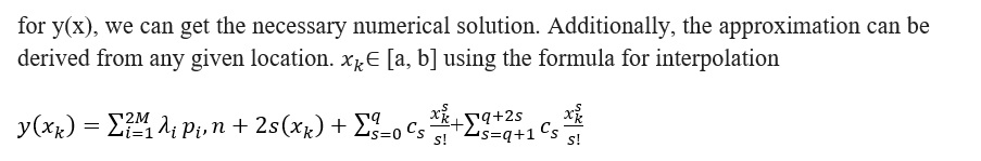 RESULTS OF CONVERGENCE ANALYSIS AND PRECISION ENHANCEMENT
 Numerical Implementation
The collocation method solves nonlinear differential equations of the form:
Precision Enhancement Techniques
- Higher-Order Basis Functions
The introduction of higher-order polynomials in the Haar wavelet basis increases the approximation capability. For example, a quadratic Haar wavelet basis is given by:
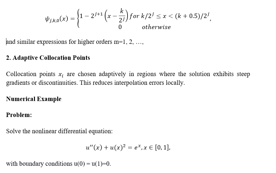
Solution Using Higher-Order Haar Wavelets:
- Approximation:
Using a 3rd-order Haar wavelet basis, approximate u(x) as:
- Abdulghani, Batool & Khorsheed, Jeeman& Mustafa Alfiky, Firas & Al-Sulaifanie, Ahmed. (2022). Haar Wavelet for Numeric Solution of Rlc Circuit Differential Equations. the journal of duhok university. 25. 1-12. 10.26682/sjuod.2022.25.2.1.
- Ahsan, Muhammad & Lei, Weidong & Ali Khan, Amir & Ullah, Aizaz & Ahmad, Sheraz & Arifeen, Shams & Uddin, Zaheer & Qu, Haidong. (2023). A high-order reliable and efficient Haar wavelet collocation method for nonlinear problems with two point-integral boundary conditions. AEJ – Alexandria Engineering Journal. 71. 185-200. 10.1016/j.aej.2023.03.011.
- Aziz I., Islam S.U., Fayyaz M. and Azram M. (2014): New algorithms for numerical assessment of nonlinear integrodifferential equations of second-order using Haar wavelets.– Walailak Journal of Science and Technology, vol.12, pp.995-1007.
- Bujurke N.M., Salimath C.S. and Shiralashetti S.C. (2008): Numerical solution of stiff systems from nonlinear dynamics using single-term Haar wavelet series.– Nonlinear Dynamics, vol.51, pp.595-605.
- Chen C.F. and Hsiao C.H. (1997): Haar wavelet method for solving lumped and distributed-parameter systems.– IEE Proc.-Control Theory Appl., vol.144, pp.87-94.
- Chertock, Alina & Levy, Doron. (2004). On Wavelet-Based Numerical Homogenization. Society for Industrial and Applied Mathematics. 3. 65-88. 10.1137/030600783.
- Arora, R. Kumar, and H. Kaur, “A novel wavelet-based hybrid method for finding the solutions of higher order boundary value problems,” Ain Shams Eng. J., vol. 9, no. 4, pp. 3015–3031, 2018, doi: 10.1016/j.asej.2017.12.006.
- Gopalakrishnan, Hariharan & Kannan, K.. (2010). Haar wavelet method for solving FitzHugh-Nagumo equation. Int. J. Math. Stat. Sci.. 2.
- Gopalakrishnan, Hariharan & Kannan, K.. (2013). An Overview of Haar Wavelet Method for Solving Differential and Integral Equations. World Applied Sciences Journal. 23. 1-14. 10.5829/idosi.wasj.2013.23.12.423.
- Hussain, Basharat & Afroz, Afroz. (2022). Haar Wavelet Series Method for Solving Simultaneous Proportional Delay Differential Equations. 10.1007/978-981-19-0179-9_25.
- Karkera, Harinakshi &Katagi, Nagaraj. (2021). Wavelet-Based Numerical Solution for MHD Boundary-Layer Flow Due to Stretching Sheet. International Journal of Applied Mechanics and Engineering. 26. 84-103. 10.2478/ijame-2021-0037.
- Kumar, Ratesh & Maan, Dr. Harpreet. (2017). Numerical solution by Haar wavelet collocation method for a class of higher order linear and nonlinear boundary value problems. AIP Conference Proceedings. 1860. 020038. 10.1063/1.4990337.
- Mohammad, Najem & Sabawi, Younis & Sh, Mohammad & Hasso, Mohammad. (2023). Haar Wavelet Method For the Numerical Solution of Nonlinear Fredholm Integro- Differential Equations. 10-25. 10.33899/edusj.2023.139892.1360.
- Qasim, Ahmed & S. Al-Rawi, Ekhlass. (2021). New Wavelet Method For Solving Partial Differential Equations. Turkish Journal of Computer and Mathematics Education (TURCOMAT). Vol.12. 3951-3959.
- Jin and Z. Luo, “A collocation spectral method for two-dimensional Sobolev equations,” Bound. Value Probl., vol. 2018, no. 1, pp. 1–13, 2018, doi: 10.1186/s13661-018-1004-0.
- Shiralashetti, Siddu & Angadi, L.M. & Deshi, A. &Kantli, Mounesha. (2016). Haar Wavelet Method for the Numerical Solution of Benjamin– Bona–Mahony Equations. 11. 136-145.
- Singh, Inderdeep. (2019). Wavelet Based Method for Solving Generalized Burger’S-Type Equations. International Journal of Computational Materials Science and Engineering. 08. 10.1142/S2047684119500209.
- Vasilyev OV, Podladchikov YY, Yuen DA. 2001. Modeling of viscoelastic plume-lithosphere interaction using adaptive multilevel wavelet collocation method. Geophys. J. Int. 147:579–89
- Verma, Amit & Kumar, Narendra & Tiwari, Diksha. (2020). Haar wavelets collocation method for a system of nonlinear singular differential equations. Engineering Computations. 10.1108/EC-04-2020-0181.
Cite this Article:
Singh, K., & Pal, R. (2025). Higher Order Haar Wavelet Collocation Method: Enhanced Precision, Convergence, and Applications to Nonlinear Differential Equations. International Journal of Applied and Behavioural Sciences (IJABS), 2(1), 147–160.
Statements & Declarations:
Peer-Review Method
This article underwent double-blind peer review by two external reviewers.
Competing Interests
The author/s declare no competing interests.
Funding
This research received no external funding.
Data Availability
Data are available from the corresponding author on reasonable request.
Licence
Higher Order Haar Wavelet Collocation Method Enhanced Precision, Convergence, and Applications to Nonlinear Differential Equations © 2025 by Kawaljeet Singh and Rajiv Pal is licensed under CC BY-NC-ND 4.0. Published by IJABS.